State dependent diversification models

Background

The goal of this post is to get the reader familiarized with state dependent diversification models. In the literature they are called state dependent speciation and extinction, because the models link the value of the states to the rates of speciation and extinction. This idea will be clearer as we work through the workshop excercises.

Note: This post is slowly evolving so materials will be changing over time.

Introduction to Bayesian Statistics and inference

For background infromation about some basic Bayesian statistics and MCMC algorithm to obtain posterior distribution samples plese reafer to the the slides below. This slides are from a short intro workshop I taught in Botany 2018 (Rochester, MN).

Bayesian stats slides here
Markov chain Monte Carlo (MCMC) slides here

Really good lecture from Paul Lewis is available in this video.

Introduction to Continuous Time Markov Chains (CTMC)

Continuous time Markov chains are our power tools when we are trying to model any discrete trait evolution in a phylogeny. CTMCs are stochastic processes, that is a random variable that we follow throughout time that is measuring the outcome of interest.

The slides below are from the Botany workshop in 2018

Continuous Time Markov Chains slides here

but more complete information can be found in this long lecture that I taught in the Midwest Phylogenetic comparative methods workshop in 2019

CTMC lecture.
RevBayes code mk2.Rev

State Speciation and Extinction Models

Here you will find all the materials about state speciation and extinction models (SSE). Most of the post is mine but there is work from of Dr. Daniel Caetano and Carrie Tribble who helped me teach the SSE models workshop at the Stand-alone SSB meeting 2020, at Gainesville, FL.

Binary state speciation and extinction model (BiSSE). A brief introduction

You will find some slides here from the Botany workshop in 2018. However, I more detailed explanation of BiSSE using RevBayes is found below.

BiSSE is a stochastic process that is the composition of two different birth-death stochastic processes connected by a transition rate. The key assumption of a BiSSE model is that the trait can be categorize in two states, each state with its own birth rate \(\lambda\) and death rate \(\mu\) representing the splitting of a lineage or the extinction of a lineage respectively. This is a big assumption because the implication is that the accumulation (or the lack of) of lineages is link to the value of the state (0 or 1) but nothing else.

Often in the literature, including the original BiSSE article, the model is represented graphically by circles and arrows connected as the figure shown below.

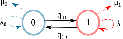
Figure 1. BiSSE graphical representation in most published papers. Trait is assumed be be binary, parameters \((\lambda_0, \lambda_1)\) are speciation rates link to each of the states, and parameters \((\mu_0,\mu_1)\) are extinction rates. The transition rates \((q_{01},q_{10})\) indicate how often the value of the trait changes.

The reason why this model is often represented as “circles and arrows” is because it is much easier to communicate than the mathematical representation. The mathematical representation behind BiSSE model is based on stochastic differential equations (known also as Kolmogorov forward equations). The goal of the equations is to define in “instantaneous time” (like a derivative) exactly what precedes the origination of a clade that is either in state value 0 or state value 1 in a very very short time frame.

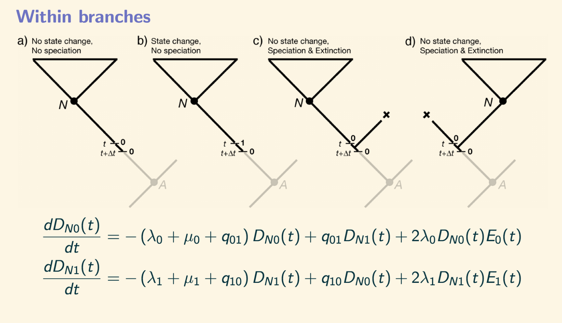Figure 2. Stochastic differential equations that define speciation in BiSSE

Why is it important to know about these equations?

Let’s just dig deeper into the interpretation of the equations shown in Figure 2. For example, the first equation defines what needs to happen for a clade \(N\) to be descendent from a lineage with state 0. The three possibilities are: 1) before time \(t\) nothing happened, the lineage was 0 and there wasn’t any speciation, nor extinction, nor a transition from 0 to 1. So the very first part of the equation \((\lambda_0+\mu_0+q_{01})D_{N_0}(t)\) represents the instantaneous probability of nothing happening. (2) There was a transition from 1 to 1 with instantaneous probability \(q_{01}D_{N_1}(t)\). (3)There wasn’t a transition of state but a speciation event \(\lambda_0\) with one lineage going extinct \(E_0(t)\) whereas the other lineage gave rise to the clade \(N\) with instantaneous probability \(D_{N_0}(t)\). Notice tha only one thing can happen at a time, either a state change or a diversification but not both simultaneously. This is one of the requirements to correctly define the model mathematically, since we are looking an infinitesimal small time interval \((t, t+\Delta t)\) the probability of two things happening exactly at the same time is zero.

These equations jointly with the equations of extinction (not shown here) are solved numerically to obtain full probabilities (not the “instantaneous” part) in any computational software building SSE models (i.e. diversitree, hisse, Revbayes). As you can imagine with more states these equations get complex quickly (see ChromoSSE for example), so bigger models are harder and harder to fit.

Another key point here is that in the definition of these equations you can see the interplay between speciation and extinction. It is difficult to discuss the speciation resulting in a clade \(N\) without talking about the extinction of a lineage. This is going to become really really important when we are estimating and interpreting diversification parameters.

BiSSE using RevBayes

Another way to think about SSE models that is not only the circle and arrow diagrams, or the stochastic differential equations themselves is the graphical model representation. The goal of this introductory workshop is to get you thinking about graphical representations because you can create custom and more complex models without having to build complex equations every time.

We will discuss some of the caveats as well at the end, but one very important key feature to clarify here is that the graphical model is not only a visual representation, but an alternative to writing the math from the model and the inference (Bayesian) simultaneously.

Rev Language Just a brief reminder that we will be using Rev language and every assignation we use has a meaning in the graphical model world. For more details please refer to (Hoehna et al. 2013 ) 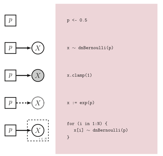Figure 3. From Hoehna et al. 2013. Rev language and its graphical model representation

Trait data utilized for the workshop Polimoneaceae data from Landis, J. et al. 2018. This is a phylogenetic tree of Phlox with selfing and outcrossing data as breeding system binary trait. We will use this dataset as an example of binary trait that could be interesting for diversification.

Trait data .csv, and phylogenetic .tre

Reading data and basics

Default for Revbayes options

setOption("useScaling","true")

For BiSSE the number of states is 2 (binary) and then we read the data. I have a folder called basicdata right where the ./rb executable is. You can specify any directory but I like to keep it there for tests. Running in the cluster I have very specific files.

NUM_STATES = 2
### Read in the data
observed_phylogeny <- readTrees("basicdata/poleult.tre")[1]
data <- readCharacterDataDelimited("basicdata/pole_datadis.csv",
stateLabels=2,
type="NaturalNumbers",
delimiter=",",
headers=TRUE)

# Get some useful variables from the data. For example taxa names in the phylogeny
taxa <- observed_phylogeny.taxa()
### Create the fix parameter for the age of the root set to the observed age
root_age <- observed_phylogeny.rootAge()

Indices that are going to be very useful for the proposals of the MCMC and for the monitors (statistics) that we are going to obtain from the inferential process (MCMC). This is not immediatly evident but it will be once we print the full model.

# Setting up indices
mvi = 0
mni = 0

Speciation and extinction rates

Now we are going to define our speciation and extinction rates. This is the part where the graphical model thinking starts helping with. We need to create four parameters \((\lambda_0, \lambda_1, \mu_0,\mu_1)\) to define speciation and extinction rates under BiSSE. Because our inferential approach is based on Bayesian statistics, what we want is to define four randon variables (r.v.s) that have a probability density function. The paradigm in Bayesian statistics states that parameters are unknown and random meaning that they have a probability distribution, since speciation and extinction rates can take continuous values, we call those probability densities, and one can choose from any density where the parameter values are positive (no negative rates allow). There are plenty of options (see here. In this example we will choose a log-Normal distribution for all four parameters of speciation and extinction, but you can and should explore other possibilities.

## Create the constant prior parameters of the diversification rates
## Number of surviving lineages is 165

mx=(ln(165/2)/observed_phylogeny.rootAge())
sx= 0.01
rate_mean <- exp(mx+sx^2)
rate_sd <- exp(2*mx+sx^2)*exp(sx^2-1)

for (i in 1:NUM_STATES) {

### Create a lognormal distributed variable for the diversification rate
log_speciation[i] ~ dnNormal(mean=rate_mean,sd=rate_sd)
log_speciation[i].setValue( rate_mean )
speciation[i] := exp( log_speciation[i] )
moves[++mvi] = mvSlide(log_speciation[i],delta=0.20,tune=true,weight=3.0)

### Create a lognormal distributed variable for the turnover rate
log_extinction[i] ~ dnNormal(mean=rate_mean,sd=rate_sd)
log_extinction[i].setValue( rate_mean )
extinction[i] := exp( log_extinction[i] )
moves[++mvi] = mvSlide(log_extinction[i],delta=0.20,tune=true,weight=3)

}

In graphical modeling what we are doing is connecting fixed with stochastic nodes that have a log-Normal distribution.

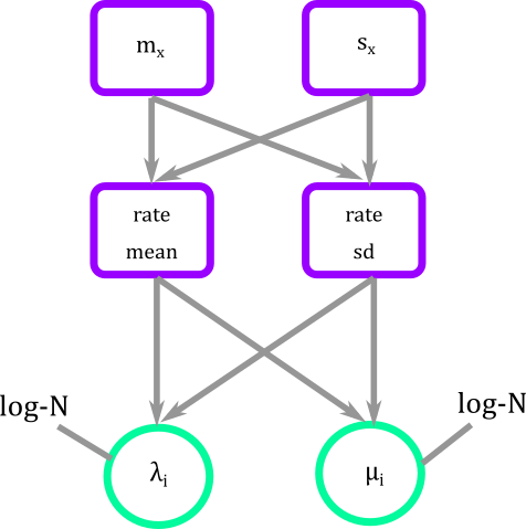
Figure 4. Graphical modeling of diversification rates of BiSSE. Squares represent deterministic nodes, circles represent stochastic nodes

Why going through so much trouble defining the log-normal as a prior distribution instead of the normal or something else?

Here is my reasoning to define these priors for speciation and extinction, yours might differ. From Nee et al. 1994 the expected number of lineages \(n\) under a simple birth-death process at time \(t\) is \(n=e^{(\lambda-\mu)t}\). That means that an expected net diversification rate \((\lambda-\mu)=\frac{ln(n)}{t}\). Now, because we condition to start with two lineages then the net diversification ends up being \(m_x=\frac{(ln(n)/2)}{t}\) with some standard deviation \(s_x\) we would like.

We could move forward and simply define \(speciation\sim N(m_x, s_x^2)\) but one caveat of doing that is that this normal could end up with negative values(!!!). So the better way to define it is via the log-speciation as a Normal distribution. One thing that comes handy here is that if we want speciation alone to have \(m_x\) as expected value, the parameters of the logNormal \((m_y, s_y^2)\) can be defined as follows \(m_y=e^{(m_x+1/2s_x^2)}\) and \(s_y=e^{(2m_x+s_x^2)}e^{(s_x^2-1)}\). Those two parameters is what you see defined in the code for all speciation and extinctions.

Transition rates

The two parameters that are missing in this discussion are the transition rates \((q_{01},q_{10})\) to connect the evolution between the states. Those parameters also need prior distributions. In this case I decided to model them using a Gamma distribution that has two parameters (a shape and a rate parameter). The way I define it is very loosely, I really don’t know how many times outcrossers and selfers have evolved in this system so I’d rather leave it this way. However, if you know something about the number of times the states have evolved from other studies, it is wise to make the mean of the Gamma distributions something that represents that knowledge (see alternative definition if I know there have been 10 transitions).

#########################################################
# Set up the transition rate matrix for observed states #
#########################################################
## I defined very loosely my gamma priors for transition rates
shape_pr := 0.5
rate_pr := 1
############### Alternative definition or rate parameter
# Each transition rate between observed states are drawn
# from an exponential distribution with a mean of 10
# character state transitions over the tree.
# rate_pr := observed_phylogeny.treeLength() / 10

q_01 ~ dnGamma(shape=shape_pr, rate=rate_pr)
q_10 ~ dnGamma(shape=shape_pr, rate=rate_pr)

moves[++mvi] = mvScale( q_01, weight=2 )
moves[++mvi] = mvScale( q_10, weight=2 )

######################################################################
# Create the rate matrix for the combined observed and hidden states #
######################################################################
rate_matrix := fnFreeBinary( [q_01, q_10 ], rescaled=false)

Again, in graphical modeling we connect fixed with stochastic nodes that have a gamma distribution, and later construct rate_matrix node that is a deterministic node, that is a function of stochastic nodes (dotted circle).

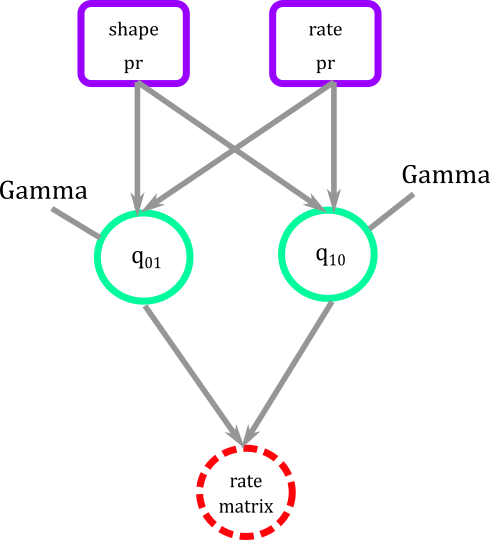
Figure 5. Graphical modeling of transition rates for BiSSE. Squares represent deterministic nodes, circles represent stochastic nodes

What are the moves? By now you would have noticed that every time I define a prior distribution I add a line of code called moves. Moves are the proposals for the Markov chain Monte Carlo (MCMC) algorithm that we are going to use to explore the posterior distribution of the BiSSE model parameters.

The moves are telling the MCMC how to explore the parametric space and are also known as proposals. For example mvSlide is a slide move, meaning that at each step of the MCMC is telling the log-speciation to slide to the left or to the right a little bit to find a new value. The mvScale tells the parameter to be rescaled. There are many many moves available in RevBayes, some specific for certain types of inferences and some others very general.

I consider selecting moves one of the hardest parts of doing inference. The moves you select have a strong influence on how quickly the MCMC will converge (or not converge). Although, there are many scientists studying convergence of MCMC algorithms, practical implementations, especially in phylogenies are hard and require a lot of patience and testing.

Treatment of the root

This is a point of great difference amongst computational packages. diversitree packagefor example allows for a weighted likelihood calculation for the frequencies of the root. hisse package has a lot more options, from using the same approach of the weyn the future I will expand more about these differences but for now I will only focus on what RevBayes is doing.

In RevBayes, we assume that the probabilities of the potential values of the root \((\pi_0,\pi_1)\) are unknown and they form a random vector. This means that we also need to estimate those probabilities. So what will do is create a prior distribution for the root that is Dirichlet because it has two important properties: 1) the values of the vector are between (0,1), and (2) the entries of the vector add to 1.

For example, values of the Dirchlet distribution can be (0.487,0.513), meaning that the root could have a value of 0 with probability 0.487 and a value of 1 with probability 0.513. Notice, that this is the only distribution so far that is multivariate. Again, we finish by defining a move in this case a multivariate one to make a proposal for the whole vectormvDirichletSimplex.

### Create a constant variable with the prior probabilities of each rate category at the root.
rate_category_prior ~ dnDirichlet( rep(1,NUM_STATES) )
moves[++mvi] = mvDirichletSimplex(rate_category_prior,tune=true,weight=2)

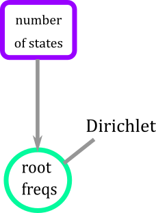
Figure 6. Graphical modeling of the root for BiSSE model. Root has a Dirichlet distribution that is a function of the number of states of the trait.

Sampling bias

Again, this is another detail of great difference in comparative methods software. At the moment, in RevBayes the only correction that can be done is to input the proportion of total observed lineages compared to the number that we should expect in the phylogeny. Other software can actually correct by sampling bias by state (see Goldberg and Igic, 2012). What approach is better?- We don’t know.

### Rho is the probability of sampling species at the present
### fix this to 165/450
sampling <- observed_phylogeny.ntips()/450

Figure 7. Graphical modeling of the sampling bias for BiSSE model. This is simply a fixed node measuring the percentage of lineages not sampled.

Full graphical BiSSE model

As of now you have a series of fixed, stochastic, and deterministic nodes free floating as small pieces of construction blocks.

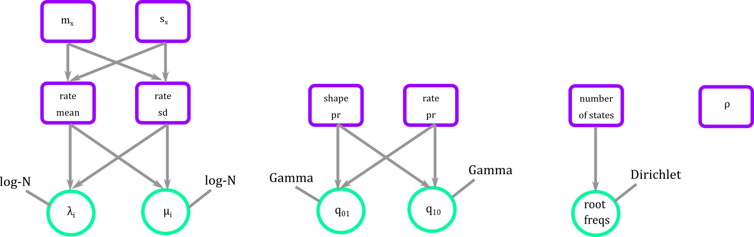Figure 8. Blocks defining the parameters that we will need for the BiSSE.

The connector is a phylogenetic distribution function dnCDBDP the character dependent birth and death process. It is in this function that we plug diversification rates, transition rates, root frequencies, and sampling to create the full BiSSE or any SSE model.

####################################################################
# Building the BiSSE Model as discrete character model+ BD process#
###################################################################

### Here is where I tie speciation, extinction, and Q using a Birth-Death with categories
bissemodel ~ dnCDBDP( rootAge= root_age,
speciationRates   = speciation,
extinctionRates   = extinction,
Q                 = rate_matrix,
pi                = rate_category_prior,
rho               = sampling )

In graphical representation the BiSSE model then looks like Figure 7.

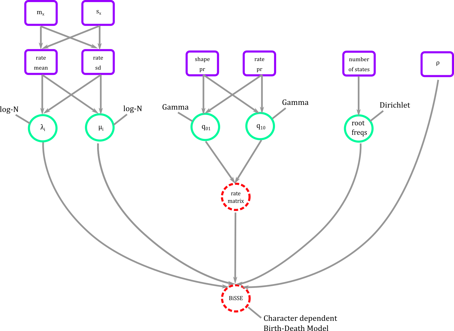Figure 9. BiSSE in graphical modeling. We connect all our modeling blocks using a phylogenetic probability distribution where diversification, transition rates, and root frequencies can be estimated.

Performing statistical inference in RevBayes

Clamping the data You might have notice that until this point we have not done anything with data other than reading it. To actually perform Bayesian statistics we need to evaluate the phylogenetic distribution that we just build (a.k.a fit BiSSE model) to the data. This happens with the help of the functions clamp that actually evaluate the dnCDBDP to the observed phylogeny and discrete character data.

### clamp the model with the "observed" tree and states
bissemodel.clamp( observed_phylogeny )
bissemodel.clampCharData( data )

In graphical model then we have added two more fixed nodes

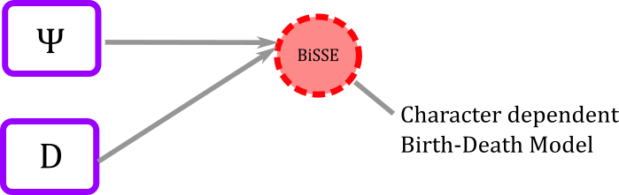
Figure 10. Clamping observed data. In the graphical model world the deterministic node of the model gets some shading to indicate that data has been clamped.

Getting what you want from the MCMC and checking the performance

In order to explore the outcome of the MCMC and also obtain posterior distributions for the model parameters monitors need to be set up. monitors as their name indicate follow the estimates throughout the MCMC generations and allow us to perform different types of inferences like ancestral state estimations and stochastic mapping.

#############
# The Model #
#############


### workspace model wrapper ###
mymodel = model(rate_matrix)

### set up the monitors that will output parameter values to file and screen
monitors[++mni] = mnFile(filename="output/BiSSE_pole.trees", printgen=1, timetree)
monitors[++mni] = mnModel(filename="output/BiSSE_pole.log", printgen=1)
##This monitor was the one giving me trouble type has to be the same that data, however I'm not hundred percent sure whether tree should be the stochastic tree assigned by the clamp or the observed_phylogeny. Will and Sebastian have different inputs

monitors[++mni] = mnJointConditionalAncestralState(tree=timetree, cdbdp=timetree, type="NaturalNumbers", printgen=1, withTips=true, withStartStates=false, filename="output/anc_states_BiSSE_pole.log")
monitors[++mni] = mnScreen(printgen=10, q_01, q_10, speciation, extinction)

Running the MCMC Finally we define a new variable mymcmc which contains all: the model you defined, the monitors, the moves of the parameters, the number of runs, and how the mcmc runs (random). We can set a number of burn-in generations (letting the MCMC find the posterior distribution) and then how many generations we actually want for the MCMC to run.

################
# The Analysis #
################

### workspace mcmc
mymcmc = mcmc(mymodel, monitors, moves, nruns=1, moveschedule="random")

### pre-burnin to tune the proposals 20% of the sample
mymcmc.burnin(generations=200,tuningInterval=50)

### run the MCMC
mymcmc.run(generations=10000)

Full RevBayes code for BiSSE bisse.Rev

RevBayes code for HiSSE hisse.Rev
Rcode for nice diversification plots

Rosana Zenil-Ferguson