
Evidential Statistics
Background
Ari Martinez spent multiple summers doing field work in the Peruvian Amazonian. In 2011, Ari observed an interesting behavior in heterospecific flocks. Depending on where on the forest a bird was feeding its response would differ. For example if a bird is feeding on the ground(dead-leaf gleaning) then the bird would “freeze” for some time, but most of the flycatchers that feed on the top of the trees wouldn’t even bother to stop.
Ari started timing the freezing behavior for some of these birds and was able to collect a small sample. He would play an alarm call and then measure the time birds were freezing depending on where they were foraging.
This is his sample and you will be using it to understand evidence in likelihood.
#Set your workind directory
#setwd(~/Dropbox/MidwestPhylo/)
bird.alarms<-read.csv("birdalarms.csv",stringsAsFactors=FALSE)
head(bird.alarms)
The model
We are going to model freezing time using an exponential distribution with parameter 1/θ, where θ is the expected time that birds of a group freeze.
The likelihood
As practiced before the likelihood function \(L(θ; X) = f(X|θ)\) is the product of the exponential density evaluated in every value of the sample observed. In R we can code it using the following function
likelihood.function<- function(parameter, observations){
probabilities <-dexp(observations, rate=1/parameter,log=FALSE)
L <- prod(probabilities)
return(-L)
}
Please note + Input of the likelihood function + Output of the likelihood function (why is it negative?)
A mini example with a sample size of two
If we have a sample size of two birds X = 2, 10 then we know based on our calculations that the maximum likelihood estimate is the average \(\hat{\theta}=\sum_{i=1}^n x_i/n\). Therefore
mle<-(2+10)/2
However, most of the time in difficult likelihoods it is impossible to calculate exactly who the mle so we do it numerically
(likelihood.optimization<-optimize(f=likelihood.function, interval=c(0,10), observations=c(2,10)))
The function optimize is used when we have unidimensional functions
(one parameter). For multidimensional we use optim or even better
nloptr from the package with the same name.
What are the outputs?
The bird alarm example
In Ari’s example we have the dead-leaf gleaning species
dl.forager<- bird.alarms$Response[which(bird.alarms$Forage=="DL")]
and the flycatchers
f.forager<-bird.alarms$Response[which(bird.alarms$Forage=="F")] #11
Calculate the MLE for DL and F and the likelihood value evaluated at the MLE
You should be getting approximately the following values:
mle.dl= 21.06248
likelihoodval.dl=7.50118e-29
mle.f=1.181818
likelihoodval.f=2.658908e-06
So, are the flycatchers behaving differently than the dead-leaf gleaners? What is the evidence? Can we compare these likelihoods or MLEs?
Where is the evidence for different behavior?
Likelihood functions are not only about the maximum likelihood estimate. Likelihoods represent plausibility. This is represented in the full likelihood function so it is important to explore it.
We select a series of parameters and measure their plausibility for example in the interval (0, 50)
parameter.vals<-seq(0.0001,50,0.01) #creating an interval for possible values for the likelihood
long<-length(parameter.vals)
# Evaluating the likelihood for each of those values
p.likelihoodf<-rep(0,long)
for (i in 1:long){
p.likelihoodf[i]<- -likelihood.function(parameter.vals[i],observations=f.forager) # Remeber is negative so we need to add a sign
}
In diffferent studies likelihood can be represented using different scales
par(mfrow=c(1,3))
# Straight likelihood function
plot(parameter.vals, p.likelihoodf, type="l",main="Likelihood for flycatchers",xlab=expression(theta),ylab="Likelihood", lwd=2,xlim=c(0,5))


#log-likelihood function, most commonly used
plot(parameter.vals, log(p.likelihoodf), type="l",main="log-likelihood for flycatchers",xlab=expression(theta),ylab="Likelihood",lwd=2,xlim=c(0,5))

# Relative likelihood: Likelihood divided by the likelihood value at the MLE
plot(parameter.vals, p.likelihoodf/likelihoodval.f, type="l",main="Relative likelihood for flycatchers",xlab=expression(theta),ylab="Likelihood",lwd=2,xlim=c(0,5))
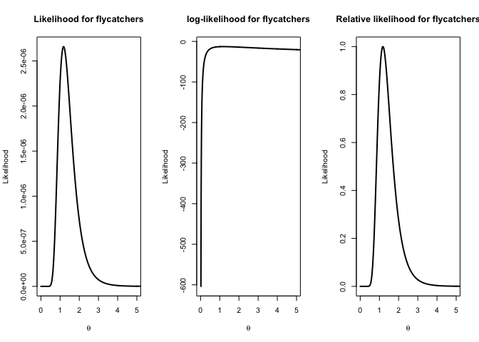
What do you think about the sample size for flycatchers?
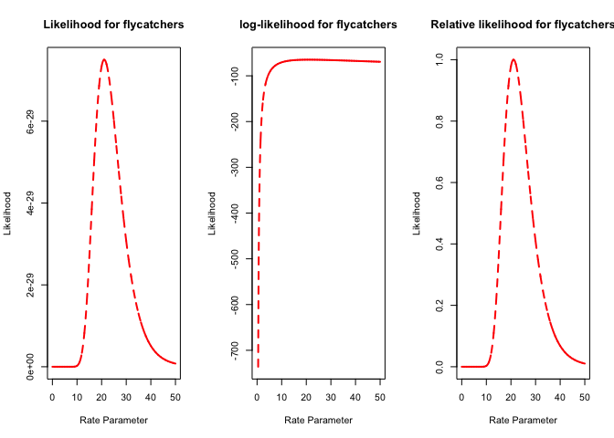
Plot the likelihood for dead-leaf gleaners
p.likelihooddl<-rep(0,long)
for (i in 1:long){
p.likelihooddl[i]<- -likelihood.function(parameter.vals[i],observations=dl.forager)
}

par(mfrow=c(1,3))
plot(parameter.vals, p.likelihooddl, type="l",main="Likelihood for flycatchers",xlab="Rate Parameter",ylab="Likelihood",lty=2,col="red",lwd=2)

plot(parameter.vals, log(p.likelihooddl), type="l",main="log-likelihood for flycatchers",xlab="Rate Parameter",ylab="Likelihood",lty=2,col="red",lwd=2)

plot(parameter.vals, p.likelihooddl/likelihoodval.dl, type="l",main="Relative likelihood for flycatchers",xlab="Rate Parameter",ylab="Likelihood",lty=2,col="red",lwd=2)
It should look like this
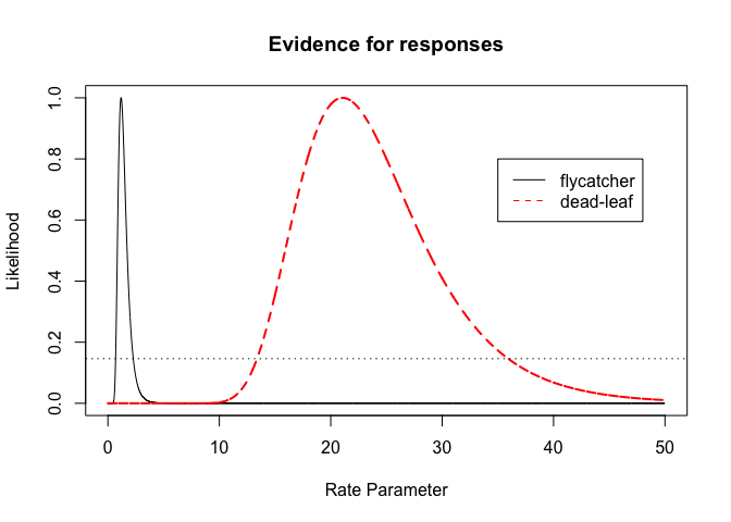
Are the freezing times different for the two groups?
Usually you will go ahead and do some statistical test to say “I reject that the average freezing time of the groups is the same”. Except that you can’t do a T-test (not normal), sample sizes are really small (so not so much power). The evidence of likelihood comes to the rescue.
Using relative likelihoods we can compare the evidence between the two groups
plot(parameter.vals, p.likelihoodf/likelihoodval.f, type="l",main="Evidence for responses",xlab="Rate Parameter",ylab="Likelihood")
lines(parameter.vals, p.likelihooddl/likelihoodval.dl,lty=2,col="red",lwd=2)
legend(x=35,y=0.8, col=c("black","red"),legend=c("flycatcher","dead-leaf"),lty=1:2)

Likelihood intervals
One very neat mathematical result (asymptotic) of using relative likelihoods is that we can cut the likelihood at 14.6% plausibility and we obtain likelihood intervals (with a large sample they become likelihood- 95%confidence inteval).
plot(parameter.vals, p.likelihoodf/likelihoodval.f, type="l",main="Evidence for responses",xlab="Rate Parameter",ylab="Likelihood")
lines(parameter.vals, p.likelihooddl/likelihoodval.dl,lty=2,col="red",lwd=2)
legend(x=35,y=0.8, col=c("black","red"),legend=c("flycatcher","dead-leaf"),lty=1:2)
abline(h=0.146,lty=3)
Likelihood ratio test
If reviewers knew more about evidential statistics they would be happy with the plot above. But Ari’s reviewers were trained in frequentist statistics so a good compromise is to use a likelihood ratio test. The statistic LRT for likelihood ratio test is calculated as LRT = − 2(logL*(*H*0) − *logL(H1))
What is the null hypothesisH0 and the alternative
hypothesis H1 in this framework? Can you calculate it using
the likelihood.function and the maximum likelihood values that we
defined above?
For the null hypothesis H0
mle.H0<-mean(c(dl.forager,f.forager))
loglike.H0<- log(-likelihood.function(parameter=mle.H0,observations=c(dl.forager,f.forager)))
Calculate the negative log-likelihood for the alternative hypothesis (You should obtain approximately)
(loglike.H1<-log(likelihoodval.f*likelihoodval.dl))
 -77.5975
Then the LRT statistic is and its p-value from a χ2 distribution with degrees of freedom 2 parameters from H1 minus 1 parameter of H0
(LRT<- -2*(loglike.H0-loglike.H1))
37.1582
(p.value<-pchisq(LRT,df=1,lower.tail=FALSE))
1.08924e-09
-
Martínez, A.E. and Zenil, R.T., 2012. Foraging guild influences dependence on heterospecific alarm calls in Amazonian bird flocks. Behavioral Ecology, 23(3), pp.544-550.
-
Strug, L.J., 2018. The evidential statistical paradigm in genetics. Genetic epidemiology, 42(7), pp.590-607.